The quickest and easiest way to lock a sheet in Google Sheets.

Locking sheets in Google Sheets is an effective way to protect your data. This article guides you on how to lock cells, rows, columns, and data ranges, and how to unlock sheets quickly and easily.

The quickest and easiest way to lock a sheet in Google Sheets.

Locking a sheet in Google Sheets is essential for protecting data and preventing unauthorized editing. This article will provide detailed instructions on how to lock cells, rows, columns, data ranges, and formulas, as well as how to unlock a sheet in Google Sheets quickly and easily.

How to quickly lock a sheet in Google Sheets

Locking an entire sheet in Google Sheets is an effective solution for protecting data, especially when you don't want others to edit the spreadsheet content. With just a few basic steps, you can easily control editing permissions. Here's how:

Step 1: Open the Google Sheets file you want to lock. On the toolbar, click Data , then select Protect Sheets and Ranges to begin setting up protection permissions.

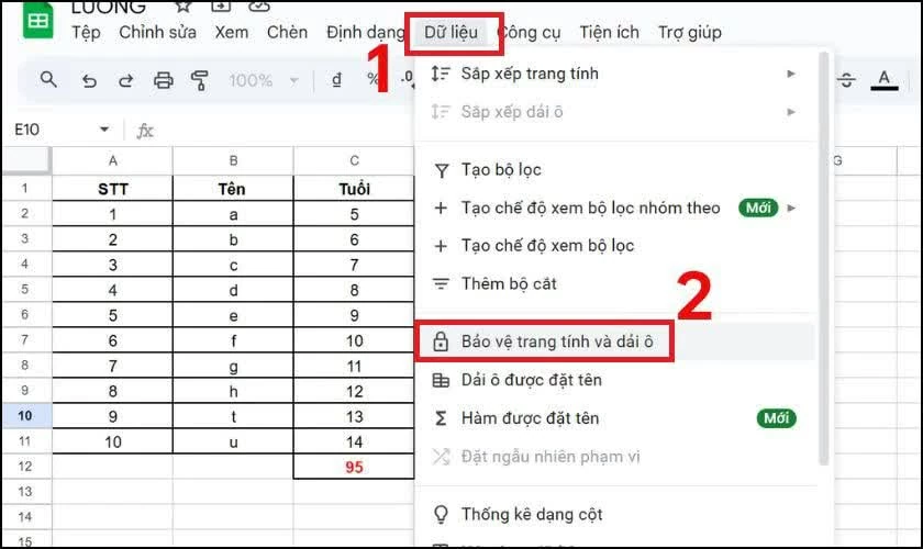Open the Google Sheets file you want to lock.

Step 2: Enter a brief description for the data area or worksheet you want to protect for easier management. Next, go to the Sheets tab, select the correct Sheet to lock, and then click Set Permissions .

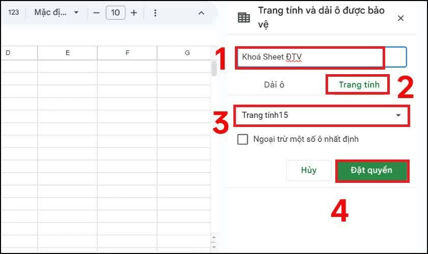Enter a brief description for the data range or worksheet you want to protect for easier management.

Step 3: Set editing permissions for the spreadsheet:

• You only : Only your account has permission to edit the content.
• Customization : Allows other people to edit by adding specific email addresses.

Step 4: After completing the settings, click Done to save the changes.

Once the above steps are completed, the entire sheet will be completely locked, or only authorized users will be able to edit it.

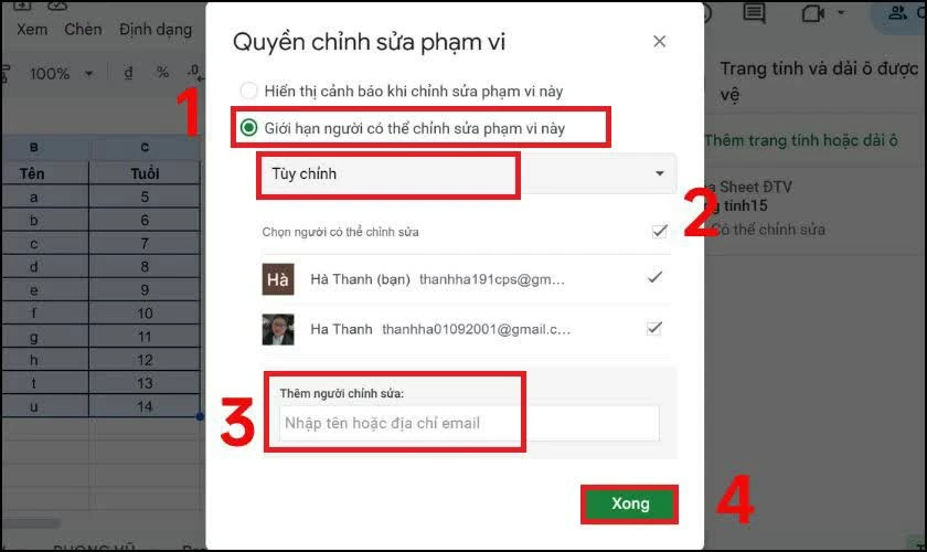After completing the installation, press Done to save the changes.

How to lock rows in Google Sheets

Locking rows in Google Sheets is a useful solution to protect important data on specific rows, especially when working with large spreadsheets or sharing files with multiple people. Locking rows minimizes unwanted changes and gives you better control over the content. Here's how to do it:

Step 1: Open your Google Sheets spreadsheet, then use your mouse to highlight the entire row of data you want to lock. On the menu bar, select Data , then click Protect Sheet and Range to begin the setup.

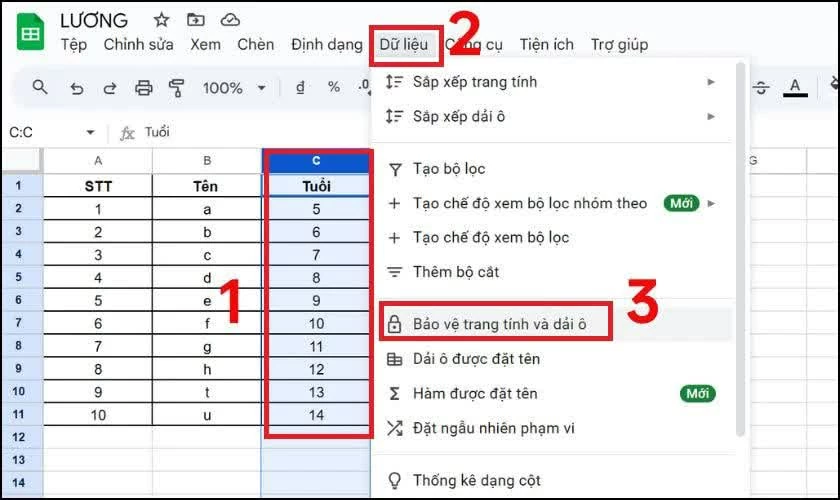Open the Google Sheets spreadsheet.

Step 2: Enter a short, memorable description for the protected area to facilitate future management. Double-check to ensure the selected area is correct, then click Set Permissions .

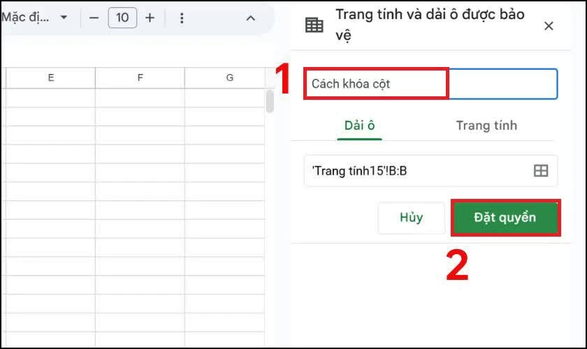Enter a short, memorable description.

Step 3: In the "Limit who can edit this range" section, select "Custom" to specify who is allowed to edit the data row. Finally, click " Done" to complete the setup process.

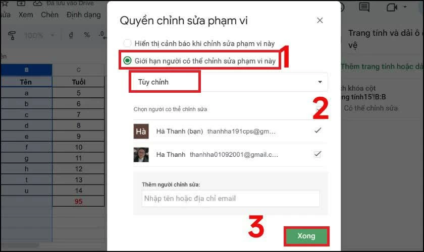In the "User Limits" section, you can edit this scope.

After completing the steps above, the data row you selected will be locked and securely protected. This helps you minimize the risk of accidental editing and ensures that important information in Google Sheets remains intact and easy to manage.

Source: https://baoquocte.vn/cach-khoa-sheet-trong-google-sheet-nhanh-chong-va-de-dang-nhat-361673.html